
 02-03-2016, 09:29 PM
|
#1 | ||
|
Pro Starter
Join Date: Sep 2009
Location: Somewhere More Familiar
|
Yet Another Excel Problem
Let's say I'm trying to run a sumif() function across a range of worksheets. I need to find value A2 on several different worksheets, and take the sum of the corresponding F column for all worksheets A2 appears on. I want something like this:
=sumif(Sheet1:Sheet5!$a:$a, $a2, Sheet1:Sheet5!$f:$f) But excel really doesn't like the syntax. I can do a simple brute force of 5 separate sumif() functions (one each for sheets 1 through 5), but there has to be a more elegant way, doesn't there? Google hasn't helped me, the numerous references to indirect() and sumproduct() do not work. |
||

|

|
|
02-04-2016, 10:33 AM
|
#2 |
|
College Prospect
Join Date: Oct 2000
Location: The Flatlands of America
|
I use something similar to what you're wanting (I think). Here is the formula that I use:
=SUMPRODUCT(SUMIF(INDIRECT("'"&Date&"'!$A$1:$A$500"),$A5,INDIRECT("'"&Date&"'!$M$1:$M$500"))) The first thing I did was select an area on my spreadsheet and created a list of each tab name I used (in this case it is 1, 2, 3,...30,31 for each day). I then highlighted the cells that had these names of the tabs, clicked on Formulas --> Name Manager, and named it Date This formula is on a summary page that lists each bus in our fleet (column A), and the miles driven for that month (column M). So in this instance, cell $A5 is bus 802. This formula goes through each tab (1-31), and sums all mileage (column M) that has bus 802 in column A. It takes into account multiple trips in a day, and does not worry about the location/order of bus 802 in cell A. Hope this helps...
__________________
Post Count: Eleventy Billion - so deal with it! Last edited by Scarecrow : 02-05-2016 at 04:04 PM. |
|
|
|
|
02-04-2016, 07:07 PM
|
#3 |
|
Pro Starter
Join Date: Sep 2009
Location: Somewhere More Familiar
|
That sounds like exactly what I'm looking for. I guess I needed to create a name for the range of my worksheets? I'm going to go check it out.
|
|
|
|
|
02-04-2016, 07:19 PM
|
#4 |
|
Pro Starter
Join Date: Sep 2009
Location: Somewhere More Familiar
|
Hrm. Still not working. If it helps, the list on each of the sheets I'm trying to pull from is full of unique names, so I'll only ever be pulling one value from each sheet to add to the sum. Here's the brute force formula I've used:
=SUMIFS('1954 Stats'!F:F, '1954 Stats'!$A:$A, $A2, '1954 Stats'!$C:$C, $C2) + SUMIFS('1955 Stats'!F:F, '1955 Stats'!$A:$A, $A2, '1955 Stats'!$C:$C, $C2) + SUMIFS('1956 Stats'!F:F, '1956 Stats'!$A:$A, $A2, '1956 Stats'!$C:$C, $C2) + SUMIFS('1957 Stats'!F:F, '1957 Stats'!$A:$A, $A2) + SUMIFS('1958 Stats'!F:F, '1958 Stats'!$A:$A, $A2, '1958 Stats'!$C:$C, $C2) This formula works, but it's ugly and inelegant. Although better than the multiple vlookup one I used before. Talk about resource hogging. I tried defining an array with 1953 Stats --> 1958 Stats and naming it Date, then using your formula above, but excel simply tells me there's a problem with the formula. It won't tell me what the problem is or what value it's returning (#N/A, #REF, etc). Last edited by Vince, Pt. II : 02-05-2016 at 10:52 AM. |
|
|
|
|
02-04-2016, 08:22 PM
|
#5 |
|
Grizzled Veteran
Join Date: Nov 2013
|
Toughie, I'd probably just keep a running total of the sum and just add to it with each new page.
__________________
"I am God's prophet, and I need an attorney" |
|
|
|
|
02-05-2016, 06:52 AM
|
#6 | |
|
College Prospect
Join Date: Nov 2006
Location: High and outside
|
Quote:
Probably not much of a help but does Excel have a problem with the spaces in the sheet names? Does it work if your sheets are "1958Stats", not "1958 Stats"? |
|
|
|
|
|
02-05-2016, 10:51 AM
|
#7 |
|
Pro Starter
Join Date: Sep 2009
Location: Somewhere More Familiar
|
That's what the ' ' are for. They denote a sheet name with a space in it.
|
|
|
|
|
02-05-2016, 12:01 PM
|
#8 |
|
College Prospect
Join Date: Nov 2006
Location: High and outside
|
Is Scarecrow's formula missing a " after $M$1:$M$500?
|
|
|
|
|
02-05-2016, 01:03 PM
|
#9 | |
|
Grizzled Veteran
Join Date: Nov 2006
Location: Backwoods, SC
|
Quote:
no its not. you are opening and closing around the ' before date and opening and clsoing aroun the !$A$1:$A$500 string |
|
|
|
|
|
02-05-2016, 02:58 PM
|
#10 | |
|
College Prospect
Join Date: Nov 2006
Location: High and outside
|
Quote:
Well, it worked for me when I put one in and tried it. It's the same quotations as the other INDIRECT statement in the formula. Last edited by Bobble : 02-05-2016 at 03:04 PM. |
|
|
|
|
|
02-05-2016, 03:17 PM
|
#11 |
|
Grizzled Veteran
Join Date: Nov 2006
Location: Backwoods, SC
|
you are absolutely right. I quoted your post about th M string and if you look at what I copied responded about the A string. WHich I totally missed
Good Catch! |
|
|
|
|
02-05-2016, 03:28 PM
|
#12 |
|
Pro Starter
Join Date: Sep 2009
Location: Somewhere More Familiar
|
Bobble, you're a genius. And Scarecrow's formula works. That's pretty awesome.
I must have looked at that for an hour last night. Not sure how it completely escaped my attention. Last edited by Vince, Pt. II : 02-05-2016 at 03:41 PM. |
|
|
|
|
02-05-2016, 04:06 PM
|
#13 | |
|
College Prospect
Join Date: Oct 2000
Location: The Flatlands of America
|
Quote:
Oops, must have deleted it when I colorized it. Fixed for future reference.
__________________
Post Count: Eleventy Billion - so deal with it! |
|
|
|
|
|
02-09-2016, 07:35 AM
|
#14 |
|
Pro Starter
Join Date: Sep 2009
Location: Somewhere More Familiar
|
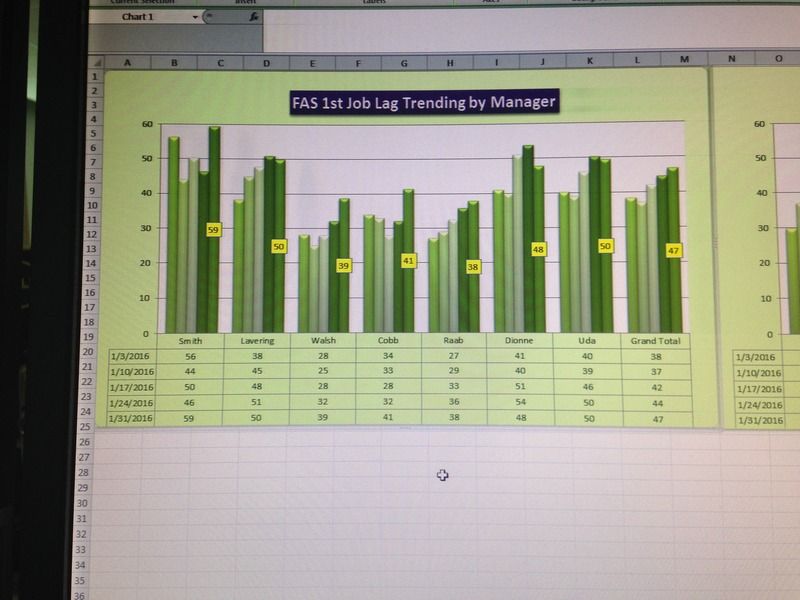
So another question: now I'm working with an inherited chart. This chart is a 2-D column chart showing five data points, sorted by date, across 7 different areas. Y-Axis is value (0-60 minutes), X-Axis is a combination of date and area: there are seven different groups of five columns, showcasing the values for the last five weeks in each area. This data comes from a simple array of date/area, with one value corresponding to each of the 35 columns in my chart.
My goal is to overlay a line graph depicting the 52-week rolling average for the area on each date. I've got the data for the average, and when I put it on a secondary axis, it overlaps just fine as columns. Unfortunately, when I change it to a line graph, it plots all of the points right on top of one another, instead of spreading them out over the 5 date values. In the series format tab, there are no options for overlap or anything like it for secondary axis series. I'll try to upload a picture to illustrate the issue, but my google-fu doesn't seem to be up to the task on this one. |
|
|
|
|
02-09-2016, 11:28 AM
|
#15 |
|
Pro Starter
Join Date: Sep 2009
Location: Somewhere More Familiar
|
 |
|
|
|
|
02-09-2016, 11:31 AM
|
#16 |
|
Pro Starter
Join Date: Sep 2009
Location: Somewhere More Familiar
|
So essentially I have another set of data that I have no problem lining up (as columns) over the top of the existing data. When I switch the new data to a line graph, instead of lining up the five data points next to one another like those columns above, it drops every single point on the same spot.
|
|
|
|
|
02-09-2016, 12:31 PM
|
#17 |
|
Pro Starter
Join Date: Sep 2009
Location: Somewhere More Familiar
|
Better photos here. Doing this from my iPhone sucks. First photo - overlapping columns:
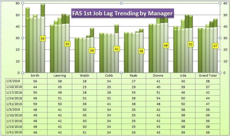 Second photo: converting to line graph: 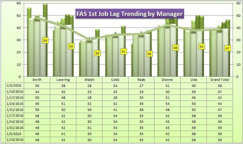 Last edited by Vince, Pt. II : 02-09-2016 at 12:35 PM. |
|
|
|
 |
| Currently Active Users Viewing This Thread: 1 (0 members and 1 guests) | |
| Thread Tools | |
|
|


